Welcome to Seeq Data Lab!

Seeq Data Lab is a rich Python-based environment for exploring and manipulating time series and industrial process data. It is built on the Jupyter interactive Python platform and Pandas data structures, making extensive use of the features and conventions that their user communities have established.

Any datasources that are connected to your Seeq Server are easy to access via Seeq Data Lab’s spy library. Several simple function calls like search, pull and push consume and/or produce DataFrames whenever possible so that you can use their powerful data manipulation capabilities and concise syntax.

This tutorial walks you through the basics of searching for data, getting it into a DataFrame and then writing it back to a Seeq Workbench workbook.

Getting Started

This section will walk you through searching for signals in Seeq and pulling data.

Importing the SPy Module

The SPy module (short for Seeq PYthon) is what you’ll use to interact with Seeq Server and access data. Start by importing it.

from seeq import spy

It’s important to set spy.options.compatibility in your script to the current major version of SPy so that you minimize the chance that a SPy version upgrade breaks your notebook or script code. By telling SPy what version you have been using and have tested with, it can make choices about what behavior is most likely to be compatible.

spy.options.compatibility = 192

You’ll also want to import Pandas so that you can work with the DataFrame structures that the spy library consumes/produces.

import pandas as pd

Logging in to Seeq

If you are using Seeq Data Lab, then this step is NOT necessary. If you are using the SPy module with Anaconda, AWS SageMaker, Azure Notebooks or any other Jupyter Notebook solution, you will need to execute this step.

Create a file in the root folder of your Jupyter project called credentials.key and put your username on the first line and your password on the second.

If you log in to Seeq Server using your corporate credentials (aka “Single Sign-On”), please take a look at the spy.login documentation for information about logging in with an Access Key.

spy.login(url='http://localhost:34216', credentials_file='../credentials.key', force=False)

Searching for Signals

Now let’s find some data. We’re going to use the built-in Seeq example data to retrieve a few signals and look at them as DataFrames.

First we’ll use the spy.search() function to retrieve metadata.

results = spy.search({
    "Path": "Example >> Cooling Tower 1 >> Area A"
})

# Print the output to the Jupyter page
results

Refining the Results

Let’s pare down the results to just three signals before we pull some data.

my_signals = results.loc[results['Name'].isin(['Compressor Power', 'Temperature', 'Relative Humidity'])]
my_signals

Now let’s pull in the data using Seeq. The data can come from any connected datasource, including historians like OSIsoft PI, time series stores like InfluxDB, and SQL databases like Microsoft SQL Server.

You can specify the grid parameter to control the granularity of the data. Seeq’s calculation engine will interpolate as needed to produce a uniform DataFrame. Specify grid=None if you want the raw data.

my_data = spy.pull(my_signals, start='2019-01-01', end='2019-01-07', grid='30min', header='Name')
my_data.head()

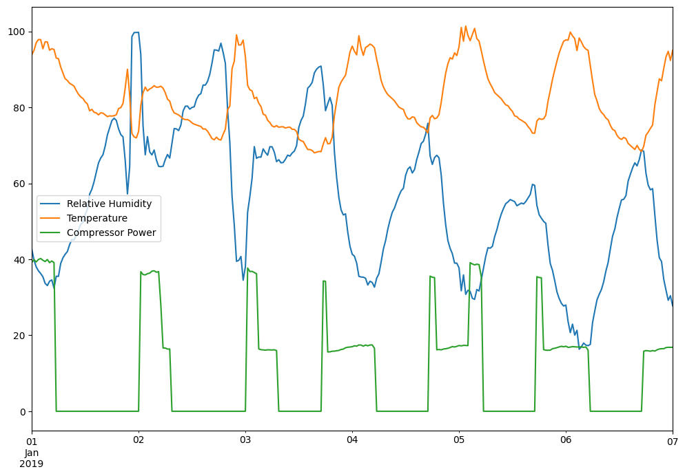
Plotting the Results

Let’s take a quick peek at the data we just pulled using the built in DataFrame.plot() function.

import matplotlib
import matplotlib.pyplot as plt

# Make the plot render at a bigger size than default
matplotlib.rcParams['figure.figsize'] = [12, 8]

my_data.plot()

<AxesSubplot:>

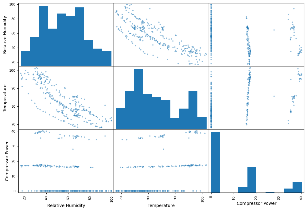
How about a matrix of scatterplots, with each variable plotted against each other? Pandas can do that easily.

pd.plotting.scatter_matrix(my_data)
plt.show()

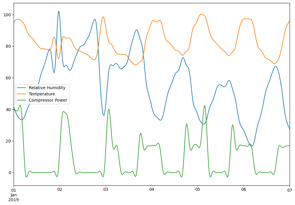
Using Seeq’s Calculation Engine

What if we want to use Seeq’s calculation engine to reduce the noise in the Temperature and Relative Humidity signals?

We can apply a calculation by specifying a formula as the calculation argument.

calculated_data = spy.pull(
    my_signals,
    start='2019-01-01',
    end='2019-01-07',
    calculation='$signal.lowPassFilter(200min, 3min, 333)',
    grid='5min',
    header='Name')
calculated_data.head()

calculated_data.plot()

plt.show()

Pushing a New Condition to Seeq

Let’s push a Seeq Condition into our workbook.

push_results = spy.push(metadata=pd.DataFrame([{
    'Name': 'Compressor on High',
    'Type': 'Condition',
    'Formula': '$cp.valueSearch(isGreaterThan(25kW))',
    'Formula Parameters': {
        # Note here that we are just using a row from our search results. The SPy module will figure
        # out that it contains an identifier that we can use.
        '$cp': results[results['Name'] == 'Compressor Power']
    }
}]), workbook='SPy Documentation Examples >> Tutorial')

push_results

Pulling the Capsules

capsules = spy.pull(push_results, start='2019-01-01', end='2019-01-07')
capsules

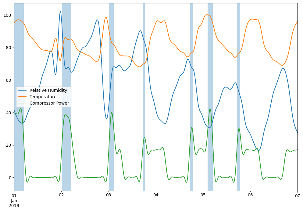
Plotting Conditions Alongside Signals

Now let’s use the new condition in a plot, this time using spy.plot(), which has a set of predefined plot configurations.

samples = calculated_data

spy.plot(samples=samples, capsules=capsules)

Calculating a New Signal using Python

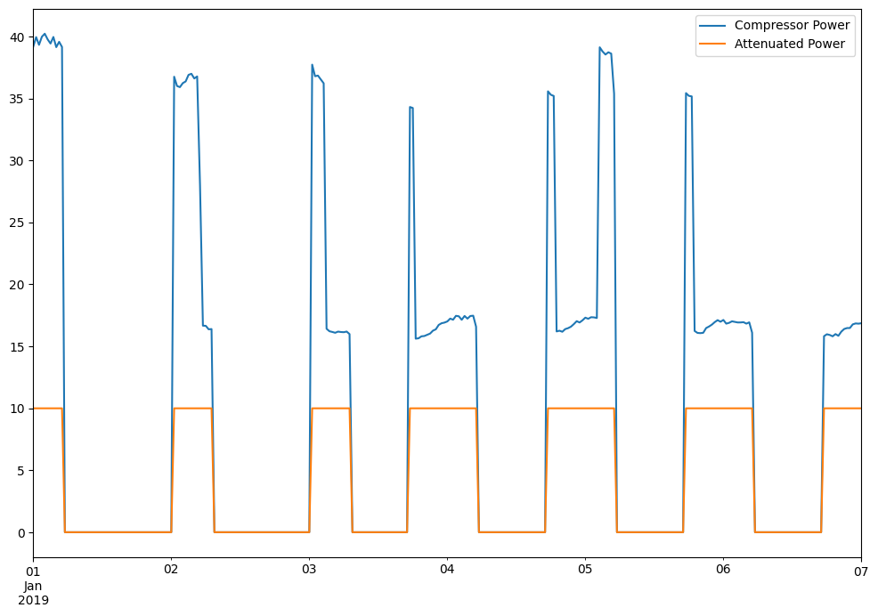
One reason you wanted to get the data into Python in the first place is to create new data. Let’s clip Compressor Power by 10 so it simplifies to just representing power on or off.

def attenuate_power(sample):
    return min(sample, 10)


clipped_data = pd.DataFrame({'Compressor Power': my_data['Compressor Power'],
                             'Attenuated Power': my_data['Compressor Power'].apply(attenuate_power)})
clipped_data.head()

clipped_data.plot()

<AxesSubplot:>

Pushing Data Into Seeq

Jupyter is a great environment for programming, but let’s go back to Seeq Workbench and make things truly interactive.

spy.push(clipped_data, workbook='SPy Documentation Examples >> Tutorial')

The data is now in Seeq’s internal time series database and is scoped to a workbook. Click the link above to see it!